XGBoost (eXtreme Gradient Boosting) is a machine learning tool that achieves high prediction accuracies and computation efficiency. Since its initial release in 2014, it has gained huge popularity among academia and industry, becoming one of the most cited machine learning library (7k+ paper citation and 20k stars on GitHub).

I was first introduced to XGBoost by one of my good friends back in 2017, the same time as I started to work on some Kaggle competitions. XGBoost quickly became my go-to approach as often times I could achieve reasonable performance without much hyperparameter tuning. In fact, XGBoost is the winningest method in Kaggle and KDDCup competitions during 2015, outperforming the second most popular method neural nets [1].

Earlier this year, I had a chance to write decision trees and random forests from near scratch. It was amazing that the math behind tree-based methods is so neat and "simple", yet the performance could be very good. I was able to go for an extra mile, managing to build a simple implementation of XGBoost. To do so, I had to study the original paper of XGBoost in depth (I probably only touched 30% of the details). I feel it is a good time to revisit what I have learned during the process.

Note that various tree boosting methods exist way before the invention of XGBoost. The major contribution of XGBoost is to propose an efficient parallel tree learning algorithm, and system optimizations, which combined together, resulting in a scalable end-to-end tree boosting system. The making of XGBoost not only requires understanding in decision trees, boosting, and regularization but also demands knowledge in computer science such as high-performance computing and distributed systems.

I will go over the basic mathematics behind the tree boosting algorithm in XGBoost. Most of the materials are referenced directly from the XGBoost paper. I'm writing this blog to strengthen and further my understanding of XGBoost, and at the same time to share my view of the algorithm.

Decision trees and gradient tree boosting

We will follow the notation from the paper. Consider a dataset with $n$ examples and $m$ features $\mathcal{D} = \{({\bf x}_i, y_i)\} (|\mathcal{D}|=n, {\bf x}_i \in \mathbb{R}^m, y_i \in \mathbb{R})$. Let $\mathcal{F} = \{f({\bf x})=\mathcal{w}_{q({\bf x})}\}(q: \mathbb{R}^m \rightarrow T, \mathcal{w} \in \mathbb{R}^T)$ denote the space of regression trees, where $T$ is the number of leaves in the tree, $q$ represents a possible structures of the tree that maps ${\bf x}$ to the corresponding leaf index, $\mathcal{w}$ is the leaf weight given the observation ${\bf x}$ and a tree structure $q$. A key step of any decision tree algorithms is to determine the best structure $q$ by continuously splitting the leaves (binary partition) according to certain criterion, such as sum of squared errors for regression trees, gini index or cross-entropy for classification trees. Finding the best split is also the key algorithm for XGBoost. In fact, all algorithms listed in the paper are related to split finding. The resulting split points will partition the input space into disjoint regions $R_j=\{  {\bf x} | q({\bf x}) = j\}$ as represented by leaf $j$. A constant $\mathcal{w}_j$ is then assigned to leaf $j$, that is $${\bf x} \in R_j \Rightarrow f({\bf x}) = \mathcal{w}_j.$$ Thus $f({\bf x})$ can also be expressed as $f({\bf x}) = \sum_{j=1}^T \mathcal{w}_j I(q({\bf x}) = j)$ which is equivalent to $f({\bf x})=\mathcal{w}_{q({\bf x})}$.

Now we can represent a tree ensemble model as a sum of $K$ additive tree functions: $$\begin{equation}   \hat y_i = \phi({\bf x}_i) = \sum_{k=1}^K f_k({\bf x}_i), \quad f_k \in \mathcal{F},   \label{eq:additive} \end{equation}$$ where each $f_k$ corresponds to an independent tree structure $q$ and leaf weight $\mathcal{w}$. The optimal tree structures and weights are then learned by minimizing the following object. $$\begin{equation}   \mathcal{L}(\phi) = \sum_{i} l(\hat y_i, y_i) + \sum_k \Omega(f_k),   \label{eq:object} \end{equation}$$ where $\Omega(f) = \gamma T + \frac{1}{2} \lambda ||\mathcal{w}||^2$ is a regularization term to penalize complex models with exceedingly large number of leaves and fluctuant weights to avoid over-fitting.

The boosting tree model can be trained in a forward stagewise manner [2]. Let $\hat y_i^{(t)}$ denote the prediction of instance ${\bf x}_i$ at the $t$-th iteration, by $\eqref{eq:additive}$ and $\eqref{eq:object}$, one needs to solve $f_t$ to minimize the following: $$\begin{equation} \mathcal{L}^{(t)} = \sum_{i=1}^n l(y_i, \hat y_i^{(t-1)} + f_t({\bf x}_i)) + \Omega(f_t). \label{eq:stagewise} \end{equation}$$ It is quit straightforward to calculate the $\mathcal{w}_j$ given the regions $R_j$. On the contrary, finding the best $R_j$ which minimize $\eqref{eq:stagewise}$ could be a very difficult task for general loss functions. To find an approximate yet reasonably good solution, we first need to find a more convenient ("easy") criterion. Here is where numerical optimization via gradient boosting comes into play. A second-order approximation of loss function was used to show that the AdaBoost algorithm is equivalent to a forward stagewise additive modeling procedure with exponential loss [3]. The XGBoost paper borrowed this idea to approximate the objective $\eqref{eq:stagewise}$ by $$\begin{equation} \tilde{\mathcal{L}}^{(t)} \simeq \sum_{i=1}^n [g_i f_t({\bf x}_i) + \frac{1}{2} h_i f_t^2({\bf x}_i)] + \Omega(f_t), \label{eq:stagewise1} \end{equation}$$ where $g_i=\partial_{\hat y_i^{(t-1)}} l(y_i, \hat y_i^{(t-1)})$ and $h_i=\partial_{\hat y_i^{(t-1)}}^2 l(y_i, \hat y_i^{(t-1)})$ are first and second order gradient, and the constant term $l(y_i, \hat y_i^{(t-1)})$ is omitted.

Given $R_j$ or equivalently $q$, from $\eqref{eq:stagewise1}$, the paper shows the optimal weight $\mathcal{w}_j^*$ in $f_t({\bf x_i})$ can be expressed as $$\begin{equation} \mathcal{w}_j^* = -\frac{\sum_{i \in R_j} g_j}{\sum_{i \in R_j} h_j + \lambda}, \label{eq:w} \end{equation}$$ and the corresponding optimal value is $$\begin{equation} \tilde{\mathcal{L}}^{(t)} (q) = -\frac{1}{2}\sum_{j=1}^T \frac{(\sum_{i \in R_j} g_j)^2}{\sum_{i \in R_j} h_j + \lambda} + \gamma T. \label{eq:obj} \end{equation}$$

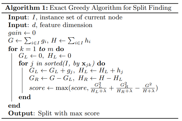
Another difficulty for finding the optimal tree structure $q$ is that the possible ways of partition the input space is numerous. Hence, the second approximation is to use a greedy algorithm that starts from a single leaf and iteratively adds branches to the tree. This is a very common approach same as the recursive binary partitions adopted in CART [2]. Let $\tilde{\mathcal{L}}^{(t)} (R_j) = \frac{(\sum_{i \in R_j} g_j)^2}{\sum_{i \in R_j} h_j + \lambda} + \gamma$, $\eqref{eq:obj}$ can be decomposed as $\tilde{\mathcal{L}}^{(t)} (q) = -\frac{1}{2}\sum_{j=1}^T \tilde{\mathcal{L}}^{(t)} (R_j)$ which means the splitting can be processed independently across all leaves (parallelism!). Consider $R_L$ and $R_R$ as the disjoint left and right regions after splitting region $R$. Then the loss reduction after the split is given by $$\begin{align} \mathcal{L}_{split} = & \frac{1}{2}\left[{\mathcal{L}}^{(t-1)} (R) - {\mathcal{L}}^{(t)} (R_L) - {\mathcal{L}}^{(t)} (R_R) \right]\nonumber\\ = & \frac{1}{2}\left[ \frac{\sum_{i \in R_L} g_j}{\sum_{i \in R_L} h_j + \lambda} + \frac{\sum_{i \in R_R} g_j}{\sum_{i \in R_R} h_j + \lambda} - \frac{\sum_{i \in R} g_j}{\sum_{i \in R} h_j + \lambda} \right] - \gamma. \label{eq:split} \end{align}$$ The best split point will then be the one resulting in the largest value of $\eqref{eq:split}$. An exact greedy algorithm of finding the split point is given as follows.

 

Besides the regularized objective mentioned in $\eqref{eq:object}$, two additional techniques are used to further prevent overfitting. The first technique is to shrink the weight update in $\eqref{eq:w}$ by a factor $\eta$, oftentimes also called a learning rate. (Recall the benefits of shrinkage methods such as ridge regression or Lasso.) The second technique is column (feature) subsampling, a technique used in Random Forest to improve the variance reduction of bagging by reducing the correlation between the trees.

$\texttt{R}$ $\texttt{gbm}$ comparison

Notice the XGBoost algorithm is different from the Gradient Tree Boosting Algorithm MART [4] showed in the ESL book. The MART is also used in the $\texttt{R}$ $\texttt{gbm}$ package [2] besides Adaboost. Let's take a closer look at the weight update equation $\eqref{eq:w}$. Define $I_j=\{i|{\bf x}_i \in R_j\}$ as the instance set of leaf $j$ and $|I_j|$ as the cardinality of $I_j$. Suppose we fix the $R_j$ and ignore the regularization term, we can express $\eqref{eq:w}$ as $$\begin{equation*} \mathcal{w}_j^* = -\frac{\frac{1}{|I_j|}\sum_{i \in I_j} g_j}{\frac{1}{|I_j|}\sum_{i \in I_j} h_j}. \end{equation*}$$ The nominator and denominator can be considered as the estimated first and second-order gradient over $R_j$ with respect to $\hat y^{(t-1)}$, the latest (accumulated) leaf weight. Does this formulation look familiar? It resembles Newton's method in convex optimization where the update is subtracting the first-order gradient divided by the Hessian matrix (like the one used for solving logistic regression but in a non-parametric fashion). The MART method is using the steepest gradient descent with only first-order approximation. As a result, we can expect XGBoost has a better quadratic approximation and have a better convergence rate to find the optimal weight (in theory).

An example with logistic regression for binary classification

XGBoost can be used to fit various types of learning objectives including linear regression, generalized linear models, cox regression, and pairwise ranking [5]. Here we will briefly discuss how to derive the weight update in $\eqref{eq:w}$ for logistic regression.

Let $y_i$ denote the binary response 0 or 1 for the $i$th observation $\bf x_i$. Let $y_i^{(t)}$ denote the accumulated weight for $\bf x_i$ after the $t$th iteration, that is $y_i^{(t)} = y_i^{(t-1)} + \mathcal{w}_j^{*(t)}$ where $\mathcal{w}_j^{*(t)}$ is the update given in $\eqref{eq:w}$ with $i \in R_j$. We will hide the superscript of $t$ from now on. By the logit link function, we have $p_i = \frac{1}{1+e^{-\hat y_i}}$ as probability estimate for $y_i = 1$.

For logistic regression, the "coefficients" are estimated based on maximum likelihood. More specifically, we will choose to minimize the negative log-likelihood function in $\eqref{eq:object}$ as $$\begin{align} l(y_i, \hat y_i)  & = -y_i \log p_i - (1-y_i) \log (1 - p_i) \nonumber \\ & = -y_i \hat y_i + \log (1 + e^{\hat y_i}). \nonumber \end{align}$$ The first and second order gradients immediately follows: $$\begin{equation*} g_i = -y_i + \frac{1}{1+e^{-\hat y_i}} = -y_i + p_i \mbox{ and } h_i = \frac{e^{-\hat y_i}}{(1+e^{-\hat y_i})^2} = p_i(1-p_i). \end{equation*}$$

We can then use the exact greedy algorithm to find all splitting points and partition the input space into $R_j$s. Finally, calculate the corresponding $\mathcal{w}_j^*$ based on the gradient information derived above.

Conclusion

In this post, we briefly go over the key algorithm in XGBoost to find the splitting points in boosting trees. The idea is behind quadratic approximation on the loss function, and the resulting algorithm and weight update are intuitive and straightforward. Without a doubt, the exact greedy algorithm discussed here alone is not good enough for a system with "eXtreme" in its name. What happens when the data is too large to be fit into the memory? Can we scale the algorithm using parallel and distributed computing? How do we efficiently store and process a sparse dataset? All the answers can be found in the second half of the paper with more implementation details in the Author's presentations and of course, the Xgboost repository on GitHub. Although some of the related system and computation topics are beyond my current knowledge, it is definitely worth trying to understand the basic tools and ideas. I hope I could make a follow-up post to discuss high-performance computing concepts used in XGBoost when I feel more confident in the subject in the near future.

References

[1] T. Chen and C. Guestrin. XGBoost: A Scalable Tree Boosting System. In Proceedings of the 22nd ACM SIGKDD International Conference on Knowledge Discovery and Data Mining, pages 785-794, 2016.

[2] T. Hastie, R. Tibshirani, and J. Friedman. The elements of statistical learning: data mining, inference, and prediction. 2nd ed. New York: Springer.

[3] J. Friedman, T. Hastie, and R. Tibshirani. Additive logistic regression: a statistical view of boosting. Annals of Statistics, pages 337-407, 2000.

[4] J. Friedman. Greedy function approximation: A gradient boosting machine. Annals of Statistics, pages 1189-1232, 2001.

[5] XGBoost Documentation